Understanding grid_weights and the L2(mu) norm

library(MetaHunt)
set.seed(1)

What `grid_weights` does

MetaHunt represents every study-level function by its values on a shared grid x_1, ..., x_G. Distances between two functions f and h are computed in a weighted L^2 sense:

||f - h||^2  =  sum_j  w_j * ( f(x_j) - h(x_j) )^2

The vector w = grid_weights is exactly that vector of weights — one non-negative number per grid point. It defines the measure mu that the inner product

<f, h>_{L^2(mu)}  =  sum_j  w_j * f(x_j) * h(x_j)

is taken with respect to. Every routine in MetaHunt that talks about “distance between functions” or “norm of a function” — basis hunting, constrained projection, conformal pointwise scores — uses the same grid_weights you supply.

When the default is fine

The default is grid_weights = NULL, which inside the package becomes the uniform vector rep(1 / G, G). Every grid point counts equally.

This is the right choice when the grid itself is a representative sample from the population whose functional you care about. For example, if you sub-sampled the grid from a held-out target-population cohort with build_grid(), the empirical distribution of the grid already encodes the target measure, and uniform grid_weights simply averages over that empirical distribution.

In short: if your grid was sampled from population P and you want distances to reflect P, leave grid_weights = NULL.

When non-uniform `grid_weights` matter

You should override the default when the grid distribution does not match the population whose distances you care about. Two common scenarios:

The grid was sampled from a source population (or a public reference like NHANES) but you want distances to reflect a target population. Pass grid_weights proportional to the target density evaluated at each grid point.
You care about a sub-region of covariate space (e.g. only patients with age > 65). Set grid_weights[j] to 0 outside the sub-region and to the target density inside.

grid_weights does not need to sum to 1 — only its relative magnitudes matter inside dfspa() and project_to_simplex(). The default wrapper in apply_wrapper() divides by sum(grid_weights), so weighted means come out on the natural scale regardless of normalisation.

A worked comparison: uniform vs non-uniform

Here we generate the same data twice — m = 40 studies, G = 30 grid points — and run dfspa() with two different grid_weights. The first run is uniform; the second up-weights the right half of the grid by a factor of about 5.

m <- 40
G <- 30
x <- seq(0, 1, length.out = G)

# True bases on the grid.
basis <- rbind(sin(pi * x), cos(pi * x), x)

# Mixing weights driven by two latent covariates.
W <- data.frame(w1 = rnorm(m), w2 = rnorm(m))
beta <- cbind(c(1, -0.8), c(-0.5, 1.2), c(0, 0))
eta  <- as.matrix(W) %*% beta
pi_true <- exp(eta) / rowSums(exp(eta))

F_hat <- pi_true %*% basis + matrix(rnorm(m * G, sd = 0.05), m, G)
dim(F_hat)
#> [1] 40 30

Now the two grid_weights choices:

gw_uniform <- rep(1 / G, G)

# Up-weight x > 0.5 by ~5x. Renormalisation is optional but tidy.
gw_right   <- ifelse(x > 0.5, 5, 1)
gw_right   <- gw_right / sum(gw_right) * G   # comparable scale, optional

fit_unif  <- dfspa(F_hat, K = 3, grid_weights = gw_uniform, denoise = FALSE)
fit_right <- dfspa(F_hat, K = 3, grid_weights = gw_right,   denoise = FALSE)

# Index sets selected can differ.
fit_unif$original_indices
#> [1] 28 18 14
fit_right$original_indices
#> [1] 18 28 14

A single overlay plot of the two recovered first basis functions makes the qualitative effect visible — the right-weighted run pays more attention to the right half of the grid when ranking which study is the “extreme” one to anchor:

matplot(
  x,
  cbind(fit_unif$bases[1, ], fit_right$bases[1, ]),
  type = "l", lty = 1, lwd = 2,
  col  = c("#0072B2", "#D55E00"),
  xlab = "x",
  ylab = "first recovered basis",
  main = expression(
    "Recovered first-vertex basis under uniform vs. target-weighted " ~ L^2 * (mu)
  )
)
abline(v = 0.5, lty = 2, col = "grey60")
legend("topright",
       legend = c("uniform", "up-weight x > 0.5", "x = 0.5 boundary"),
       col    = c("#0072B2", "#D55E00", "grey60"),
       lty = c(1, 1, 2), lwd = c(2, 2, 1), bty = "n")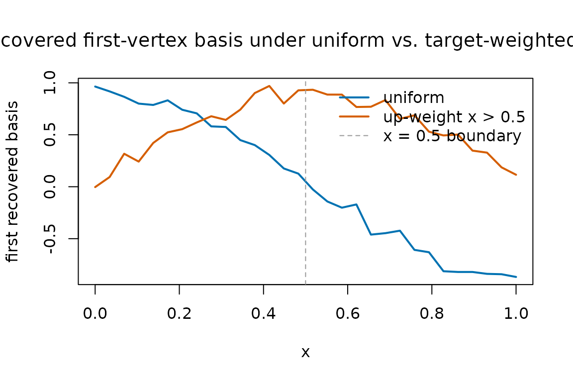

The two curves usually agree closely on the well-sampled regions and diverge where the weights differ most. The takeaway is not that one choice is right and the other wrong — it is that grid_weights quietly determines which features of the function get prioritised.

Practical guidance

Start with the default. Only switch if you have a concrete reason (target distribution, sub-region focus, deliberate down-weighting of unreliable grid points).
Make grid_weights strictly positive on the support you care about. Zero weight at a grid point removes it from every distance, norm, and mean computation in the package. This includes the d-fSPA denoising step, which uses the same L²(μ) inner product to define neighbourhoods.
Keep the same grid_weights across dfspa(), project_to_simplex(), and the conformal routines for a given analysis. Mixing different grid_weights between steps is rarely what you want — it changes the meaning of “distance” mid-pipeline.
If you only care about a scalar functional (e.g. an ATE), passing a wrapper is often a cleaner solution than re-weighting the grid. See vignette("wrapper-scalar").

Functions that accept `grid_weights`

The argument has the same meaning everywhere it appears:

dfspa(F_hat, K, grid_weights = NULL, ...)
project_to_simplex(F_hat, bases, grid_weights = NULL, ...)
apply_wrapper(F_mat, wrapper = NULL, grid_weights = NULL) — used for the default weighted-mean wrapper.
metahunt(F_hat, W, K, ..., grid_weights = NULL) — passes the weights through to dfspa() and project_to_simplex().
split_conformal(...), cross_conformal(...), conformal_from_fit(...) — all accept grid_weights for the pointwise conformity score and for the default wrapper when none is supplied.
reconstruction_error_curve(), cv_error_curve(), select_denoising_params() — propagate grid_weights to the underlying dfspa() calls.

If a function does not accept grid_weights directly, it is because it operates on already-projected weights pi_hat (e.g. fit_weight_model()) and therefore does not need the grid measure.

What grid_weights does