An introduction to MetaHunt • MetaHunt

library(MetaHunt)
set.seed(1)

The problem: function-valued meta-analysis

You have several studies — trial centres, cohorts, sites — and each one has produced a fitted model for some function of patient-level covariates. That function might be a regression curve, a CATE, or a dose-response curve. You also have study-level metadata for each study: region, sample composition, year, and so on. You want to predict that function for a new study, characterised only by its metadata, together with a prediction band, and you want to do it without ever pooling patient-level data across studies.

MetaHunt is designed for exactly that workflow. It assumes a small number of latent basis functions drive cross-study heterogeneity, recovers them from the per-study estimates, and learns how the mixing weights depend on study-level metadata. The result is a single fitted object that you can predict() for new metadata and combine with conformal prediction for uncertainty quantification. If you would rather see one short example before reading the full pipeline, start with vignette("get-started", package = "MetaHunt").

Key assumptions

The MetaHunt pipeline rests on four assumptions. We state them in applied-reader voice; the manuscript contains the formal statements and proofs.

A1. Low-rank cross-study heterogeneity

We assume the true study-level functions all live inside the convex hull of a small number $K$ of shared latent basis functions. Each study is a convex combination of the bases, with non-negative weights that sum to one. Geometrically, every study is a point inside a $(K-1)$ -simplex whose vertices are the basis functions; the bases are identifiable as the vertices of that hull.

Formally, there exist basis functions $g_1, \ldots, g_K$ with $K < m$ such that, for every study $i \in \{0, 1, \ldots, m\}$ , $f^{(i)}(\boldsymbol{x}) \;=\; \sum_{k=1}^{K} \pi_{ik}\, g_k(\boldsymbol{x}), \qquad \boldsymbol{x} \in \mathcal{X},$ with weight vector $\boldsymbol{\pi}_i = (\pi_{i1}, \ldots, \pi_{iK})^\top \in \Delta_{K-1}$ , the $(K-1)$ -simplex. The bases are non-degenerate, i.e. $g_2 - g_1, \ldots, g_K - g_1$ are linearly independent in $L^2(\mu)$ .

What this buys you: the entire $m$ -by-grid table of study functions collapses to $K$ shared shapes plus an $m$ -by- $K$ table of weights, so heterogeneity becomes low-dimensional and shareable.

A2. Weight model

The mixing weight $\boldsymbol{\pi}_i$ for study $i$ is drawn from some conditional distribution given that study’s covariates $\boldsymbol{W}_i$ . The distribution can be anything you can estimate — a Dirichlet regression, an RKHS-Dirichlet, a multinomial logit, a nearest-neighbour smoother. MetaHunt does not commit you to a specific functional form.

Formally, for $i = 0, 1, \ldots, m$ , the weight vectors are independent draws $\boldsymbol{\pi}_i \mid \boldsymbol{W}_i \;\stackrel{\text{ind.}}{\sim}\; \mathcal{P}_{\boldsymbol{\pi} \mid \boldsymbol{W}}(\,\cdot \mid \boldsymbol{W}_i),$ where $\mathcal{P}_{\boldsymbol{\pi}\mid\boldsymbol{W}}$ is an arbitrary distributional map from the covariate space $\mathcal{W}$ to the simplex $\Delta_{K-1}$ .

What this buys you: once you can map metadata to weights, predicting the function for a brand-new target population reduces to predicting its weights and re-mixing the recovered bases.

A3. Exchangeability

The studies (including the target) are exchangeable units drawn from a common data-generating process: their joint distribution is invariant under reordering. This is much weaker than i.i.d. and is the standard condition under which conformal prediction is valid.

Formally, the site-level covariates $\boldsymbol{W}_0, \boldsymbol{W}_1, \ldots, \boldsymbol{W}_m$ are exchangeable. Combined with A1–A2, this implies that the triples $\bigl(\boldsymbol{W}_i,\, \boldsymbol{\pi}_i,\, f^{(i)}\bigr), \qquad i = 0, 1, \ldots, m,$ are jointly exchangeable across $i$ .

What this buys you: the calibration step in conformal prediction inherits a finite-sample, distribution-free coverage guarantee with no need for parametric error models.

A4. Estimation error control

Each study reports a noisy version of its true function, $\hat f^{(i)} = f^{(i)} + \epsilon^{(i)}$ . We assume the within-study estimation error vanishes uniformly in the within-study sample size, and that the number of studies $m$ does not grow too fast relative to those sample sizes. In words: every study should be reasonably well-estimated, and you should not have a large number of studies whose individual sample sizes $n_i$ are small.

Formally, write $\hat f^{(i)}(\boldsymbol{x}) = f^{(i)}(\boldsymbol{x}) + \epsilon^{(i)}(\boldsymbol{x})$ . We assume $\sup_{\boldsymbol{x} \in \mathcal{X}} \mathbb{E}\!\left[\epsilon^{(i)}(\boldsymbol{x})^2\right] = O\!\left(n_i^{-r}\right) \quad \text{for some } r > 0,$ and that $m = o\bigl(\inf_i n_i^{\,a}\bigr)$ for some $0 < a < r$ , where $n_i$ is study $i$ ’s sample size.

What this buys you: the noise in $\hat F$ does not accumulate through the pipeline, basis recovery is consistent, and conformal intervals retain their asymptotic coverage despite a multi-stage estimator.

The three-step pipeline

metahunt() is a thin wrapper around three exported steps. You can also call them individually if you want fine-grained control.

Step 1. Basis hunting via d-fSPA

dfspa() extends the Successive Projection Algorithm to functions. It iteratively picks the study whose current residual norm is largest, projects the rest onto the orthogonal complement, and repeats $K$ times. A denoising step averages each study with its near neighbours before the search; this trades a small bias for substantially smaller variance when the per-study estimates are noisy.

Step 2. Fitting weight model

For each study, project_to_simplex() finds the convex weights that best reconstruct its observed function from the recovered bases. fit_weight_model() then regresses these weight vectors on the study-level covariates W using a method of your choice (default: Dirichlet regression).

Step 3. Target prediction

predict.metahunt() takes a new metadata row $W_0$ , predicts its weight vector through the fitted weight model, and returns the convex combination of the recovered bases. With wrapper = mean (or any other reduction) it returns a scalar summary — for example, an ATE under a uniform grid weighting.

A worked end-to-end example

For the rest of the vignette we work with a simulated (F_hat, W) so the truth is known. In your own data, replace this block with the data-prep onramp described in vignette("data-prep").

G <- 40; m <- 120; K_true <- 3
x <- seq(0, 1, length.out = G)
basis <- rbind(sin(pi * x), cos(pi * x), x)         # 3 true bases on the grid

W <- data.frame(w1 = rnorm(m), w2 = rnorm(m))       # study-level covariates
beta <- cbind(c(1, -0.8), c(-0.5, 1.2), c(0, 0))
pi_true <- exp(as.matrix(W) %*% beta)
pi_true <- pi_true / rowSums(pi_true)

F_hat <- pi_true %*% basis + matrix(rnorm(m * G, sd = 0.05), m, G)
dim(F_hat)
#> [1] 120  40

In real data, F_hat[i, ] would be predict(model_i, newdata = grid) and W[i, ] would be that centre’s metadata. The data-prep vignette describes a one-line lm-based onramp.

Fit the full pipeline and inspect the recovered bases:

fit <- metahunt(F_hat, W, K = 3)
fit
#> MetaHunt fit
#>   m (studies):    120 
#>   G (grid size):  40 
#>   K (bases):      3 
#>   weight method:  dirichlet 
#>   predictors:     w1, w2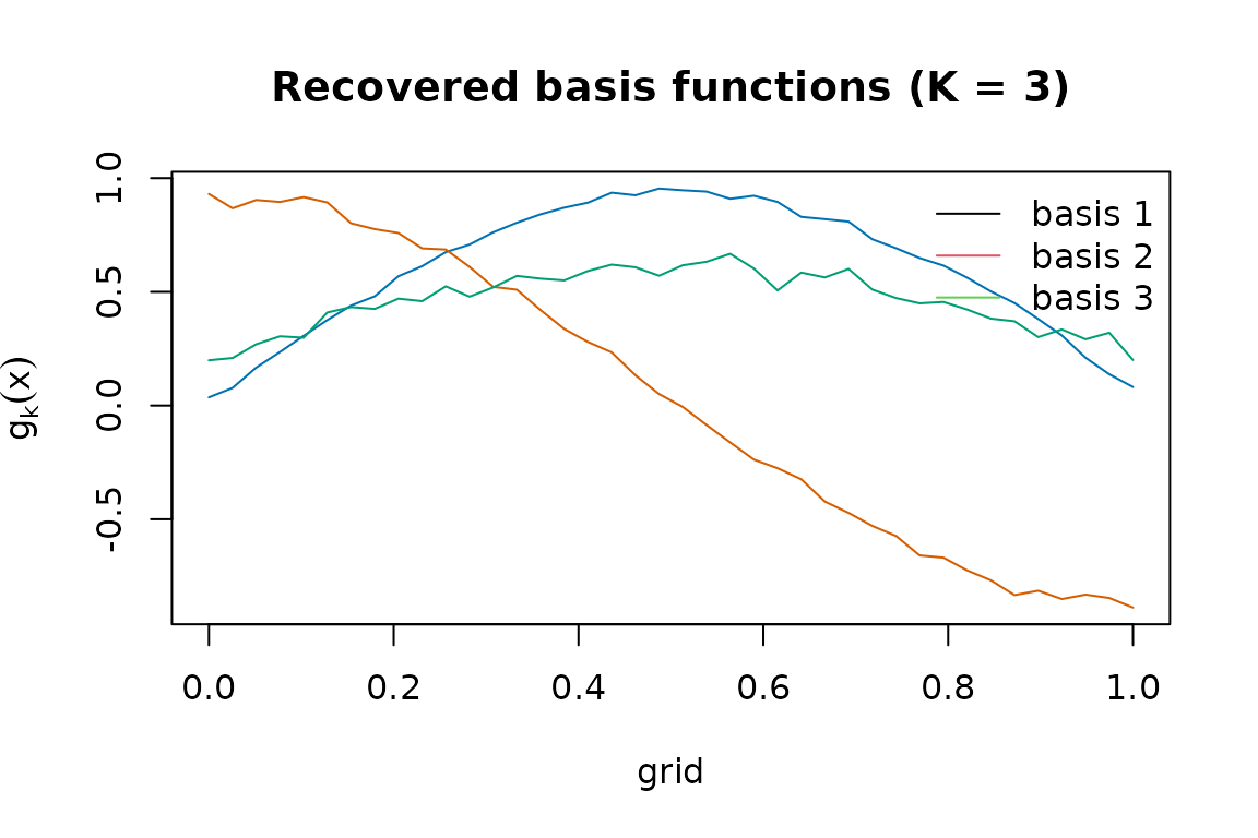

plot(fit, x_axis = x,
     col = c("#0072B2", "#D55E00", "#009E73"))

Predict the target functions for three new metadata profiles and plot them:

W_new <- data.frame(w1 = c(0, 1, -1), w2 = c(0, -0.5, 1),
                    row.names = c("baseline", "high w1, low w2", "low w1, high w2"))
f_pred <- predict(fit, newdata = W_new)
dim(f_pred)
#> [1]  3 40
oldpar <- par(mar = c(4, 4.5, 3, 1))
matplot(x, t(f_pred), type = "l", lty = 1,
        col = c("#0072B2", "#D55E00", "#009E73"),
        xlab = "x", ylab = expression(tilde(f)(x)),
        main = "Predicted target functions")
legend("topright", legend = rownames(W_new),
       col = 1:3, lty = 1, bty = "n")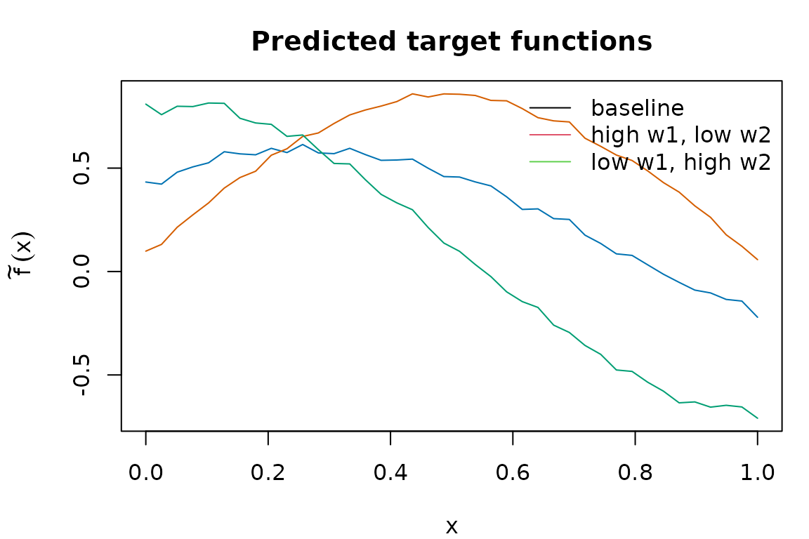

par(oldpar)

Pass a wrapper for a scalar summary per target (an ATE under uniform grid weights):

predict(fit, newdata = W_new, wrapper = mean)
#> [1] 0.3318159 0.5559631 0.1020037

Where to next

vignette("data-prep") — turning per-centre fitted models into (F_hat, W) via build_grid() and f_hat_from_models(), including a self-contained lm onramp.
vignette("grid-weights") — choosing the grid_weights argument and the underlying $L^2(\mu)$ inner product.
vignette("choosing-k-denoising") — picking the rank $K$ and the d-fSPA denoising knobs (N, Delta) via elbow and CV diagnostics.
vignette("conformal-prediction") — split, cross, and from-fit conformal bands around the target function.
vignette("wrapper-scalar") — using wrapper = mean and other reductions to turn function-valued predictions into ATEs and related scalar estimands.
vignette("minmax-baseline") — when to prefer the covariate-free worst-case-regret aggregator and how it compares to MetaHunt.
Function-level references: ?metahunt, ?dfspa, ?fit_weight_model, ?predict_target.

References

Shi, W., Imai, K., and Zhang, Y. (2024). Privacy-preserving meta-analysis through low-rank basis hunting.

Zhang, Y., Huang, M., and Imai, K. (2024). Minimax regret estimation for generalizing heterogeneous treatment effects with multisite data. arXiv:2412.11136.